Lagrange Multipliers

Consider the unconstrained optimization problem

\min_{x \in \mathbb{R}^n} ~~ f(x)

The first criteria for $x^*$ to be a local minima is that the gradient $\nabla f(x^*)$ that represents the direction of steepest ascent, becomes zero. This means, in an unrestricted space (absence of constraints) where the point $x$ can move in any direction in $\mathbb{R}^n$ in order to minimize the function, has no where to go. How to interpret the same thing in a constrained optimization problem? In this article I will try to give an intuition for this problem with the help of widely used Lagrange multipliers.

Consider the following optimization problem with equality constraint

\begin{aligned} &\min_{x \in \mathbb{R}^n} ~~ f(x)\\ &s.t. ~~~~~ h_i(x) = 0 ~~ i = 1, 2, \cdots, p \end{aligned}

Now, the decision set is restricted. The point x can not move freely in $\mathbb{R}^n$ .

1. One Equality Constraint

For simplicity, let us only consider an example with only one constraint $h$ .

\begin{aligned} &\min_{x \in \mathbb{R}^n} ~~ x^2 + y^2 + xy\\ &s.t. ~~~~~ x+y-1 = 0 \end{aligned}

The solution to this problem attains at A $= (\frac{1}{2}, \frac{1}{2})$ (DIY) as shown in the Figure 1.

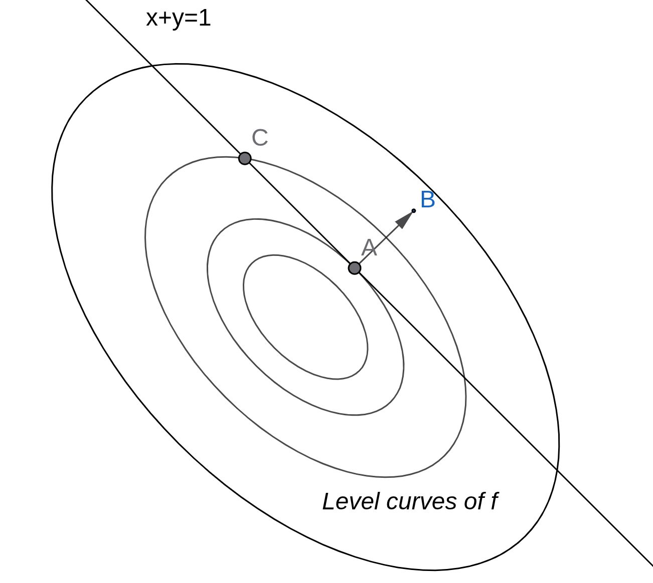
Figure 1: Contour visualization

One important thing to note in the above figure, at optimal point (A), the constraint line is a tangent to the level curve. If the constraint was non-linear, at the point of optima, the both $f$ and $g$ will have a common tangent. The intuition is that at a different feasible point say C, where the level curve intersects the constraint, if the function $f$ moves towards A, it can still reduce its value. Therefore, C can not be a optimal point.

This fact becomes more clear when we look at the normal (ray AB) to both the curves at the point A. The normal to the level curve and the constranints are parallel $i.e., \nabla_{x}f(A) = \mu \nabla_{x}g(A)$ . Notice, that the gradient of $f$ at A is not zero but the direction of steepest ascent (take negative and it becomes descent) is parallel to the normal to the gradient. Therefore, any step toward that direction will lead to constraint violation. Based on the equation given in the above equation, we define the lagrangian function as follows

L(x, \mu) \doteq f(x) + \mu g

where $\mu$ is a called a Lagrange multiplier. In $L, \mu$ acts as a penalty term for violating $g$ . We wish to stay on the constraint set $g$ and $\mu$ acts as a pushback, ensuring that any movement away from $g$ becomes undesirable in L. We solve the Lagrangian $wrt x, \mu$ , and the resultant $x^*$ is also optimal point of the original problem.

2. Many Equality Constraints

what happens when there are two equality constraint $g_1, g_2$ in the problem? A point of optima need to satisfy both the constraints. Like the one constraint case, does the level curve and two constraints share the same tangent at the point of optima? What about the normal to the level curve at an optimal point? Let us take an example by adding an new constraint $g_2: x^2 + y^2 = 4$ to our previous problem. The solution attains at $[1.82, -0.82]^T$ as shown in the figure below.

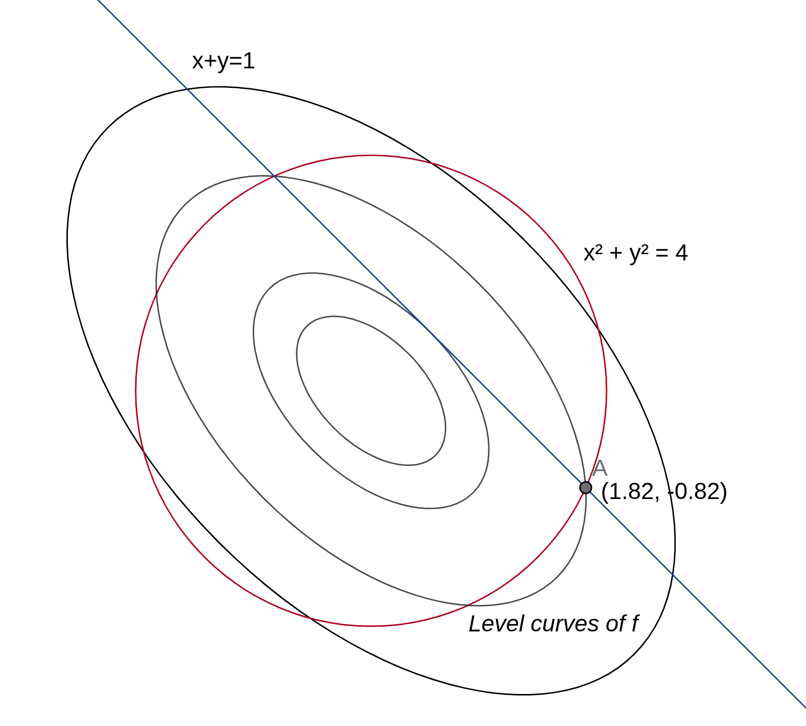
Figure 1: Contour visualization

One can see that the gradient of the objective function is not zero at $A$ . Also, the tangent to the level curve, $g_1$ and $g_2$ are not parallel anymore. The observations about the normal to the level curve is not the same but can be extended with increasing number of constraints.

The idea was that at the point of optima, the gradient should not be able to take any local step along a vector that can minimize further. Such a vector if exists (non zero) should be perpendicular to the constraints so that any step along that direction takes $f$ out of feasible region. Therefore, gradient is spanned by the normals to the constraints, i.e. $\nabla_{x}f(A) = \mu_1 \nabla_{x}g_1(A) + \mu_2 \nabla_{x}g_2(A)$ .

Therefore, extending similar argument, the Lagrangian for $p$ equality constraints problem can be written as

L(x, \mu) \doteq f(A) + \sum_{i=1}^p \mu_i g_i

3. Inequality Constraints

Inequality constraints $g_i(x) \le 0$ is called inactive $x$ if $g_i(x) < 0$ . This is called inactive because it allows local movement along all possible direction around $x$ without violating the constraint. Since, it allows local movement along all possible direction, it does not influence the optimality of the function. Therefore, while solving a optimization problem, inactive constraints are ‘ignored’. When $g_i(x) = 0$ , it mostly behave like a equality constraint with a condition that the corresponding Lagrange multiplier $\lambda_i$ is non-negative. This is because, at an optimal point $x^*, g(x^*) = 0$ and from the Lagrangian

\begin{aligned} \nabla_x f(x^*) + \lambda \nabla g(x^*) &= 0 \\ \Rightarrow \nabla_x f(x^*) &= -\lambda \nabla g(x^*) \end{aligned}

$\nabla g$ points outside the feasible region, therefore, if $\lambda < 0$ it encourages $f$ to violate the constraint, which is not a expected behaviour. The function of a constraint is to push back the function not pull outside the feasible region. For details on the role of Lagrangian multipliers in optimization of an NLP (Non-linear Programming) see the KKT condition (Write a new article on KKT conditions).

4. Interpreting Lagrange Multipliers

Lagrange multipliers are interpreted as an amount force the constraint applies at the optimum. It tells about the sensitivity of a constraint. How much does the objective function change with a unit change in the corresponding constraint. To form a mental model, if a constraint is seen as a blockade, the corresponding Lagrange multiplier tells how strongly the constraint is blocking the objective function. It also represents the importance of a constraint in shaping the gradient vector $\nabla f$ .